Approximation is expensive, but the lunch is cheap
Authors
Publication
*Produced under the mentorship of Evan Hubinger as part of the *SERI ML Alignment Theory Scholars Program - Winter 2022 Cohort.
Thank you to @Mark Chiu and @Quintin Pope for feedback.
Machine learning is about finding good models: of the world and the things in it; of good strategies and the actions to achieve them.
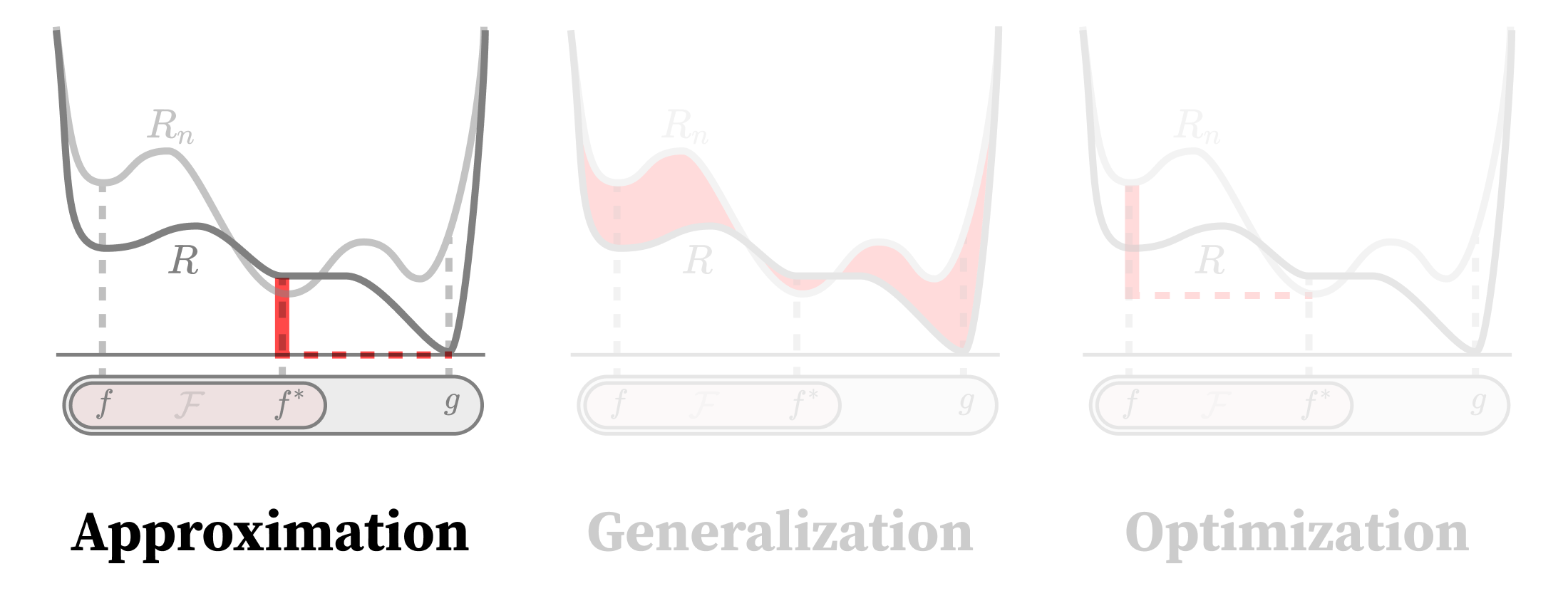
A sensible first question is whether this is even possible — whether the set of possible models our machine can implement contains a model that gets close to the thing we care about. In the language of empirical risk minimization, we want to know if there are models that accurately fit the target function and achieve low population risk, \(R(f^*)\).
If this isn’t the case, it doesn’t matter whether your training procedure finds optimal solutions (optimization) or whether optimal solutions on your training set translate well to new data (generalization). You need good approximation for “optimal” to be good enough.

The classical approach to approximation is that of universal approximation theorems. Unfortunately, this approach suffers from being too general and not saying anything about efficiency (whether in terms of the parameter count, weight norm, inference compute, etc.). It doesn’t tell us what distinguishes neural networks as approximators from any other sufficiently rich model class such as polynomials, Gaussian processes, or even lookup tables.
To find out what makes neural networks special, we have to move away from the classical focus on bounds that are agnostic to the details of the target function. You can’t separate the properties that make neural networks special from the properties that make real-world target functions special.
In particular, neural networks are well-suited to modeling two main features of real-world functions: smoothness (flat regions/low frequencies) and, for deep neural networks, sequential subtasks (hierarchical/modular substructure).
A major flaw of classical learning theory is that it attempts to study learning in too much generality. Obtaining stronger guarantees requires breaking down the classes we want to study into smaller, more manageable subclasses. In the case of approximation, this means breaking apart the target function class to study “natural” kinds of target functions; in the case of generalization, this will mean breaking apart the model class into “learnable” subclasses.
Already long underway, this shift towards a “thermodynamics of learning” is at the heart of an ongoing transformation in learning theory.
Universal approximation is cosmic waste

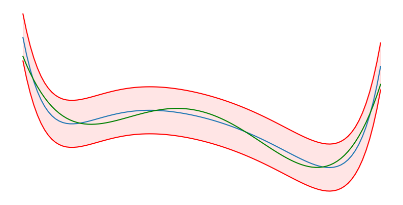
Universal approximation is about showing that you can approximate (green) a target function (blue) within a uniform bound (red) over a fixed interval.
Polynomials are universal approximators. The original universal approximation theorem dates back to Weierstrass in 1885. He proved that polynomials could “uniformly” approximate any desired continuous function over a fixed interval, where “uniformly” means that the difference between the outputs of the target function and model function is less than a fixed distance, \(\epsilon\), for every input.1
Infinite-width networks are universal approximators. Half a century later, Stone generalized the result to arbitrary “polynomial-like” function classes2 in what is now known as the Stone-Weierstrass theorem. In 1989, Hornik, Stinchcombe, and White showed that infinite-width one-hidden-layer neural networks with sigmoidal activations satisfy the conditions of this theorem, which makes neural networks universal approximators. It’s possible to obtain the same guarantees for networks with more modern activation functions (Telgarsky 2020) and through different approaches (e.g., Cybenko 1989).
Universal approximation is expensive. The main problem with these results is that they say nothing about efficiency, i.e., how many parameters we need to achieve a good fit. Rather than blanket statements of “universal approximation,” what we’re really after are relations between model class complexity (as measured by the number of parameters, weight norm, etc.) and expressivity.
There is such a thing as a cheap lunch. To derive these scaling relations, we need to make additional assumptions about the set of target functions we want to model. The non-straw-man takeaway from the no free lunch theorem is that efficient approximation requires both simple targets and expressive models. Learners can exploit the real-world, but it comes at the cost of restricting the set of things you are able to learn. The lunch ain’t free, but it sure is cheap.
Almost all functions look like this high-frequency nonsense.
We don’t care about functions that look like this.
Target-dependent approximation bounds. Barron (1993) derived one of the first relations between target functions and neural network approximation. By constraining how much the target function oscillates, Barron found that the number of hidden units required to achieve a target accuracy, \(\epsilon\), scales as \(C/\epsilon^2\). This looks like a very strong bound until you observe that the variable \(C\), which is the “Barron norm” responsible for constraining oscillations, scales exponentially with the input dimension, \(d\), and target class complexity.3 So we’re not quite there yet.
Others, like Mhaskar (1996) and Pinkus (1999) study the more general target of \(n\)-differentiable functions, \(C^n\), which leads to a correspondingly looser bound of \(\epsilon^{-d/n}\) hidden units. Generally, these results with shallow networks don’t lead to practical bounds.
Infinite-depth universal approximation. The thing is: we care about deep networks. Can we achieve better efficiency when we move past one hidden layer?
The answer is… not immediately? Yarotsky (2017) restricts his attention to modeling Sobolev functions (functions with well-defined derivatives up to some order). Sure, the depth is bounded by a much milder logarithmic bound, \(c(\ln(1/\epsilon) + 1)\), but the number of parameters is still subject to curse-of-dimensionality effects, \(c\epsilon^{-d/n}(\ln(1/\epsilon)+ 1)\). Other approaches (e.g., Gühring et al. (2019), Hanin and Sellke (2017) and Hanin (2019)) don’t fare much better.4
To obtain stronger efficiency guarantees, we have to enforce stronger restrictions on the target function class. What properties of real-world data can we take advantage of to narrow the space of target functions?
Neural networks like low frequencies
Real-world data is low frequency. In natural data, frequency is often inversely correlated with importance: locality means we don’t care about the microscopic fluctuations in a gas or the moment-by-moment ups and downs of the stock-market; we care about the macroscopic properties and long-timescale trends.5
Low frequencies are cheap. NNs learn piecewise functions (Balestriero 2018). In particular, ReLUs learn piecewise linear6 functions, which are much more efficient at fitting low frequency functions than, for example, polynomials or sinusoids. Conversely (as we saw with the Barron norm), high-frequency targets require exponentially many neurons.

The square bump. You only need a few parameters to approximate a square bump with ReLUs but dozens for polynomials and sinusoids. In addition, the out-of-domain extrapolation is much less misbehaved for the ReLU than it is for the polynomial or sinusoid.
Spectral biases. Researchers study this affinity for low-frequency data under the heading of “spectral biases,” which explain not only approximation but also generalization: if the target function does contain irrelevant high-frequency noise, neural networks will struggle to learn these, and end up generalizing better. See Rahaman et al. (2019), Yang and Salman (2019), or Xu et al. (2019).

ReLU networks fit piece-wise linear functions/decision boundaries.
Artifact of the activation. One problem with this explanation is that the spectral bias seems to be largely due to the particular choice of activation function. Hong et al. (2022) show that choosing a different activation function (the hat function) can eliminate the bias, and Tancik et al. (2020) do the same, but with a sinusoidal encoding method. Both claim that this not only maintains performance, but improves it, for some image-based tasks. So this isn’t everything.
But what does this tell us about depth? The more critical limitation this explanation is that it holds for both deep and shallow networks, so it tells us nothing about the role of depth. Smoothness may be necessary for neural networks’ success, but it’s not sufficient to explain the success of deep neural networks.
This is important! Recent work in interpretability shows us that deep neural networks appear to have significant internal machinery, implementing things like world models (Nanda 2023) or multi-step algorithms (Olsson et al. 2022; Nanda and Lieberum 2022). Shallow networks have no room for either of these things — they approximate in a single step, in much the same way that an interpolated lookup table does. So if we’re looking to explain the “magic” of modern machine learning, depth needs to play a central role.7
What is it about depth?
Let’s think step-by-step. Computer science has long realized that there are some tasks that appear to be easily parallelizable, and others which seem inherently sequential. Not every program runs faster with more cores! In the worst case, you might need exponentially more resources to simulate a sequential machine with a parallel one (see\(NC \not= P\) below). It seems natural then that the architecture we use for learning should reflect this. So maybe that’s what depth is doing?
Depth separations. We can see this through the literature on “depth separations” or “no-flattening theorems.” These involve constructing specific families of target functions that deep neural networks can approximate exponentially more efficiently than shallow networks.

We can overcome the curse of dimensionality because real problems can be broken down into parts. When this happens sequentially (like the trees on the right) deep networks have an advantage.
There is a laundry list of examples available in the literature: sawtooth functions (Telgarsky 2016), sum-product functions (Delalleau and Bengio 2011), functions with positive curvature (Liang and Srikant 2016; Yarotsky 2017; Safran and Shamir 2017), piecewise smooth functions (Petersen and Voigtlaender 2018), Gaussian mixture models (Jalali et al. 2019), polynomials (Rolnick and Tegmark 2017; Shapira 2023), model reduction models (Rim et al. 2020; Poggio et al. 2017), and efficiently solvable families of differential equations (Dahmen 2022).

Telgarsky (2016) shows that deep NNs can express sawtooths exponentially more efficiently than shallow networks (though this pattern may be too fine-scale to be learnable in practice).
Individually, these results suffer from the opposite extreme of universal approximation: they’re mostly too specific to tell us anything about realistic target functions. Toy examples can be useful, but they’re not the full picture.
Modularity and hierarchy. But if we zoom out, these results sure seem to be pointing at something. The examples share some common features: notably, a sequential or modular substructure. This is what Lin et al. (2017) refer to as “hierarchy,” what Poggio et al. (2017, 2022) refer to as “compositionality,” and what Hoang and Guerraoui (2018) refer to as “non-parallelizable logical depth.”
When are problems tractable? In order to figure out what this really means, we need to take a step back for a moment. There’s a classic problem in learning theory, known as the “curse of dimensionality”: the number of possible functions grows exponentially in the number of inputs. Consider an “easy” case: there are \(2^{2^n}\) Boolean functions with \(\)\(n\) inputs, so it takes \(2^n\) bits to specify just one. An arbitrary MNIST-size classifier would take more bits than are contained in the observable universe! Clearly the functions we care about in practice must have more structure than this.
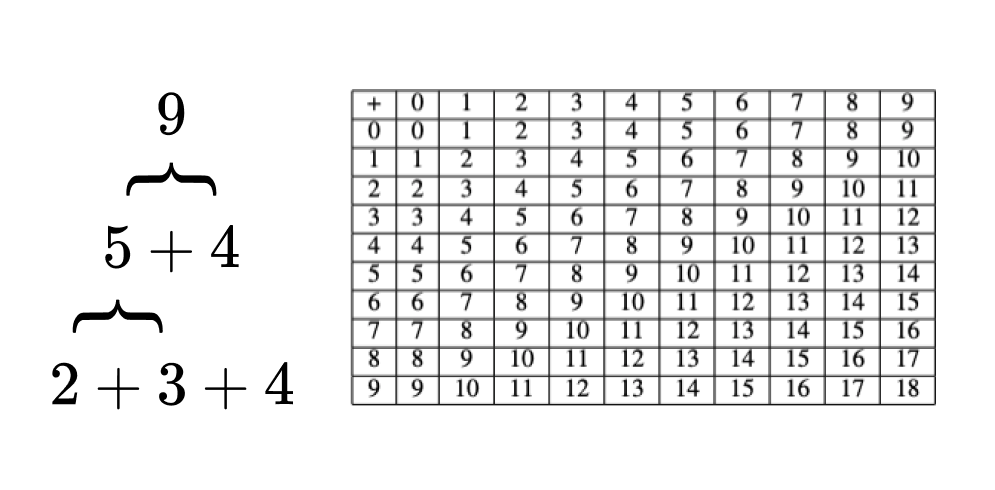
Real-world*, tractable* functions have the quality that you can solve them “piece-by-piece” and “step-by-step” — they can be built up by composing together small functions with fewer inputs. Then you only have to memorize the smaller functions and how they fit together rather than the full specification of the function’s outputs. A classic example is addition: just memorize how to add pairs of two integers together, and you can repeat this to add any number of integers you want in linear time.

Real-world functions can be solved “piece-by-piece” and “step-by-step.”
Depth and width. From this perspective, the difference between depth and width becomes clear: depth helps when the problem has sequential sub-tasks, and width helps when some of these tasks are parallelizable. Shallow networks miss out on depth, so they can’t take advantage when the underlying problem has sequential steps. They can do “piece-by-piece,” but not “step-by-step.” Vice-versa, as you might predict, skinny networks miss out on width and can’t take advantage of parallel subtasks (which Lu et al. (2017) confirm).
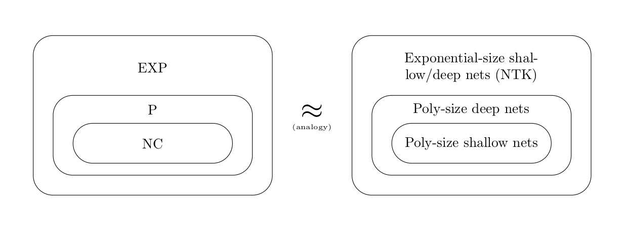
NC ≠ P. This resembles the relationship between NC and P in complexity theory (see Hoang and Guerraoui (2018)). From this perspective, it’s quite natural that Lu et al.’s (2017) bound on skinny networks is polynomial, while traditional depth separations are exponential, since sequential machines can polynomially simulate parallel ones but (assuming \(NC \not= P\)) not vice-versa.8

If you’re dealing with arbitrary functions with many inputs, your only bet is to “memorize”, which takes exponential size. But if your problem can be broken down, deep nets can do polynomial size. If your problem isn’t sequential, shallow nets can do the same.
Expressivity ≠ ease-of-learning. As we’ll see in a subsequent post on optimization, just because a neural network can express some function in theory doesn’t mean it can learn that function in practice. Several papers, such as Malach and Shalev-Schwartz (2019) or Telgarsky (2016), create fractal-like functions that deep networks can technically express more efficiently than shallow networks, but aren’t actually learned in practice. This only applies to a subset of depth separation results, but can easily become a point of confusion when reading the literature.
Recall that the advantage that depth provides is in tackling the curse of dimensionality, helping to deal with (step-by-step) functions as the number of inputs gets very large. But papers such as Malach and Shalev-Schwartz (2019) only consider functions with a small number of inputs. In a way, they’re “cheating”: you can simulate an increasing number of discrete inputs using fractals with increasing resolution. But while deep neural networks can technically do this, the pathological construction means that it’s quite rare. The average number of piecewise regions learned by a ReLU network is far smaller than the maximal number of piecewise regions expressible (Hanin and Rolnick 2019).
No approximation without assumption
Assumptions all the way down. If we take the uncharitable view, then, sure, neural networks are universal approximators, but they are exponentially expensive. And, sure, you can show a little spectral bias result here, a little depth separation there, but claiming that these toy target functions actually capture some relevant kernel of truth about real-world functions ultimately rests on forcing opportunistic assumptions onto the real-world.
Efficiency schmefficiency. More charitably, neural networks may be exponentially expensive, but who cares when VCs are willing to foot the bill? And when we take a step back to look from the trees to the forest, the depth separations sure seem to be screaming something or other about hierarchy. It may be that we can’t get to any strong efficiency results without making a few assumptions about real-world data, but, then again, learning is as much about model selection (i.e., making the right starting assumptions) as it is about inference.
Approximation ⇔ generalization ⇔ optimization. The results on spectral biases and depth separations show that it is difficult in practice to disentangle approximation from generalization and optimization. The same assumptions that lead to more efficient approximations also lead to better generalization (Kawaguchi et al. 2021). Meanwhile, efficient approximations aren’t necessarily easy to learn; the right choice of pathological target can be nigh impossible to learn even if it is expressible by the network architecture. Classical learning theory’s taxonomy of approximation, generalization, and optimization isn’t as appropriate as it first seemed.
Thermodynamics of learning. As we saw, the only way to obtain more efficient bounds was to introduce restrictions to the target function class. As we will see in the next post, to obtain stronger generalization bounds, we will need to break apart the model class in a similar way. In both cases, the classical approach attempts to the study the relevant phenomenon in too much generality, which incurs no-free-lunch-y effects that prevent you from obtaining strong guarantees.
But by breaking these classes down into more manageable subclasses, analogous to how thermodynamics breaks down the phase space into macrostates, we approach much stronger guarantees. As we’ll find out in the rest of this sequence, the future of learning theory is physics.
Footnotes
-
Cf. Taylor approximation which tells us that we can approximate any (k)-times differentiable function locally with a (k)-th order polynomials. ↩
-
(1) That is continuous, (2) that for each point there is a function that is non-zero given that input, (3) that for every two points there is a function that has different outputs on those two functions, and (4) that the function class is an algebra under the composition rule. ↩︎ ↩
-
The constant, (C), is the supremum of (2\pi\int ||x|| \cdot |f(x)|,\mathrm d x). ↩
-
Reminiscent of these results on universal approximation are proofs that certain neural networks are Turing-complete. In 1994, Siegelmann and Sontag proved this for RNNs with sigmoidal activation functions. More recently, Peréz et al. (2019) did the same for transformers with hard attention. These are stronger results than the universal approximation bounds, many of which assume continuity or smoothness: they tell us that RNNs are able to simulate arbitrary computable functions. That said, they’re subject to the same weaknesses (=efficiency). When restricted to reasonable p, transformers are rather low on the Chomsky hierarchy (Delétang et al. 2023). ↩
-
At the same time, real-world functions also definitely feature meaningful oscillations. You could argue this makes sinusoids that much more efficient than neural networks. This is the weakness of hand-wavy appeals to assumption. We counter with another hand-wavy appeal to “well but Fourier approximation sure doesn’t seem like it’s going to kill us.” ↩
-
Technically, piecewise linearity isn’t enough, since, as mentioned elsewhere, Hong et al. (2022) shows that the hat activation function (which is also piecewise linear) has no spectral bias. The difference seems to be that the bends in ReLUs aren’t “too jagged”. ↩
-
Many papers on approximation fail to distinguish the shallow case from the deep case. Much of the spectral bias literature, for instance, applies to shallow networks just as well as deep networks, but the authors frequently go on to argue that this explains the success of deep learning. This is unnecessary confusion. ↩
-
The proper analogy might instead be to equate shallow and deep networks to (\text{AC}_0) and (\text{NC}_1), respectively. In fact, the “original” depth separation results can actually be found in the literature on Boolean circuits. To avoid taking a detour into circuit complexity, we use NC and P instead. ↩
Discussion
Join the conversation on LessWrong to discuss this post with the community.